Deep Learning is at the forefront of modern artificial intelligence, enabling machines to accomplish tasks that were once the stuff of science fiction. Part of this revolution is Convolutional Neural Networks (CNNs) which help drive advancements in computer vision and image recognition. If you’ve ever been curious about how machines can recognize objects in images, you’re in the right place. In this series, we embark on exploration of CNNs, demystifying their inner workings and unveiling their applications in the realm of deep learning.

What are convolutional neutral networks?

Convolutional neural networks (or often just abbreviated CNN) are just one of the many different types of artificial neural network. They are widely used in computer vision for image recognition and image classification tasks. With the use of (relatively) simple mathematics they create a structure of interconnected neurons whose values would help them recognize different objects in an image.  They use relatively simple mathematics to figure out patterns in images and then recognize different objects inside the images. CNNs mimic the way our brains work by creating a few different sets of interconnected neurons whose values and connections reflect different patterns of an image. To make predictions, CNNs go through several steps, which include retrieving information from images (such as edges, curves, colors, etc.), which is an operation called convolution. Then any not needed information is removed using the pooling operation. After that the activation of the different neurons is calculated and the CNNs predicts which object is present in the image.

Long story short, convolutional neural networks used those so called “sliding windows” to scan the image, retrieve information from the image like edges, curves, colors, etc., then calculate the values and weights of each neuron in every hidden layer and then come up with a probability what that image is.

Convolutional neural networks perform either image classification or image recognition. In this blogpost we will cover mostly image classification, since it’s easier to grasp in terms of mathematics, but image recognition is done the same way just using different activation functions (you will see what that is in a moment) and slightly different architectures.

Furthermore, convolutional neural networks can predict more than 1 object in an image and do consider colors when performing all the calculations, but for the sake of simplicity today we will use as an example only grayscale images with a single object in them.

The convolution operation

Now let’s take a ride through the process of how convolutional neural networks set their weights and values so that they can recognize different objects. The convolution operation (or also known as “feature extraction”) is the very first starting point of image recognition when it comes to CNNs. What this operation does is to simply slide a window (a kernel, or also known as filter) over the image so that we can get only specific features of the image. This window slides 1 pixel (sometimes 2 or 3) at a time going from left to right and top to bottom to retrieve specific features of the image such as curves, lines, etc.

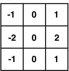
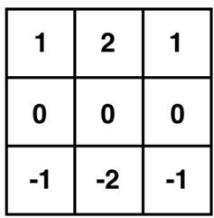
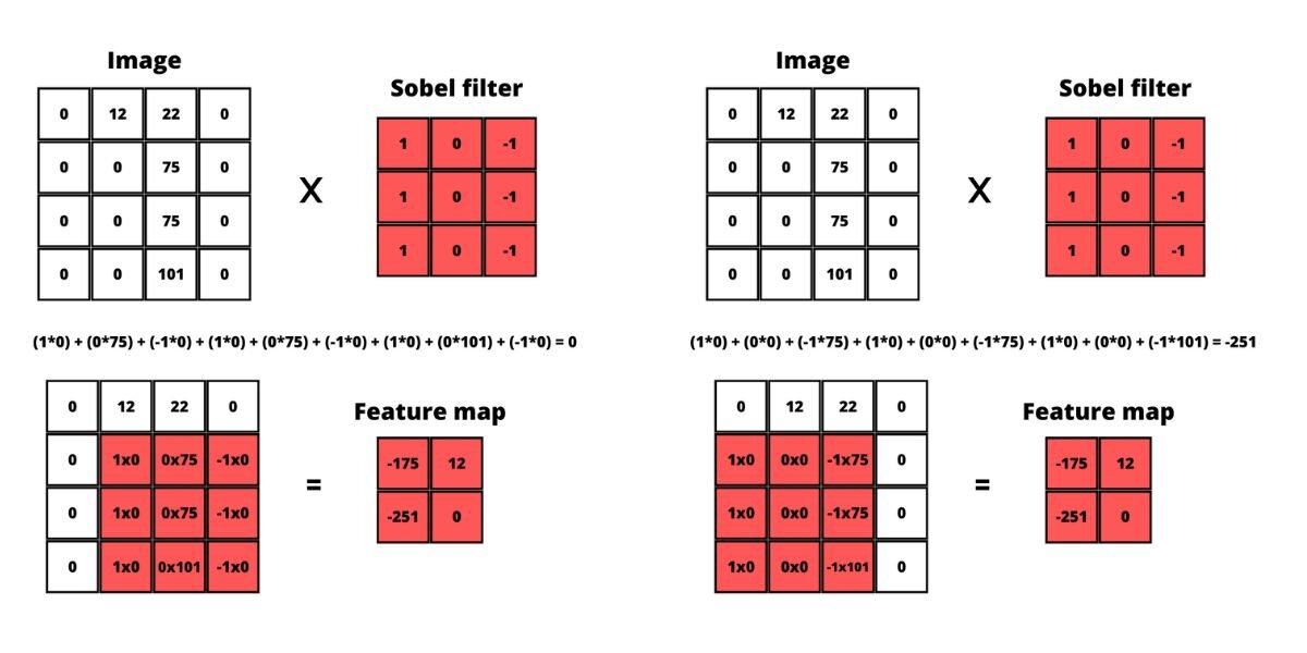
Let’s take as an example the Sobel filter. A well-known example for such filter is the Sobel filter which can be used for retrieving vertical or horizontal edges from the image. Below you can see visualization of a kernel with a vertical and horizontal Sobel filter with a size 3×3 pixels. 

Image Source

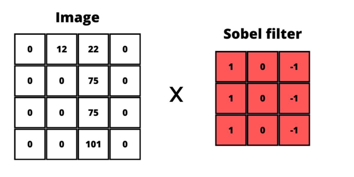
What happens is this 3 by 3 filter is the so-called sliding window that usually starts at the very top of the image (0,0) and goes through the whole image 1 pixel at a time. Each pixel is multiplied by the corresponding value from the filter. E.g. here is how applying the Sobel filter changes an image: 

Image source

For this example, a grayscale image is used because then the values of each pixel would be a single value between 0 and 255 (0 is black and 255 is white). When we are working with colorful images then this multiplication is performed on each of the color channels (red, green, and blue) separately.

So how does all that help in image recognition? Only the vertical edges wouldn’t be sufficient, so a bunch of other filters, like Gabor Filter, Gaussian Filter are applied to the image to extract specific features.

The Convolution operation output

The output of this convolution operation is usually referred to as feature map. If we take for example an image of 4×4 pixels (which isn’t much of a real-world scenario, but still) and we apply a 3×3 filter to it, then a 2×2 feature map will be created. If we want to produce a feature map with the same size as the image, we should just wrap the image with 0 pixels around it. We could also produce an even smaller feature map by using a larger stride. Stride is a parameter in the convolutional layer that describes the number of pixels the sliding window would go through. By default, it is 1 pixel, but we can set a stride of 2 which means that the sliding window would slide by 2 pixels.

Here’s a visual representation of a sliding window over a bunch of random grayscale pixels.

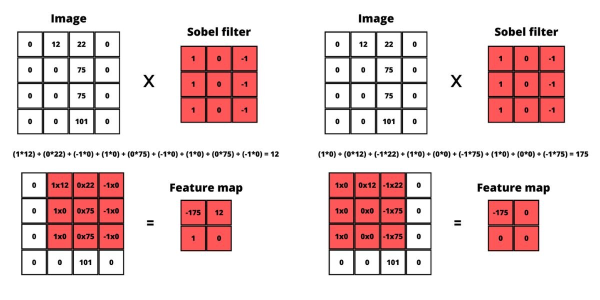
When applying filters, we want to apply not just one, but multiple filters and then we will stack (or concatenate) them together. Stacking means just combining the feature maps together into a 1-dimensional array. Each filter generates a separate feature map that represents a specific feature or pattern detected in the input image.

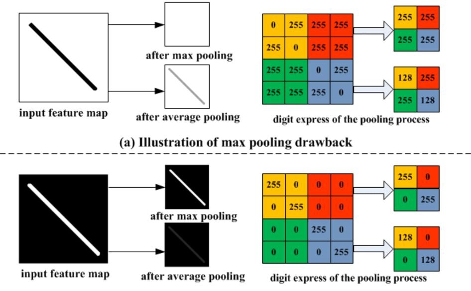
Pooling

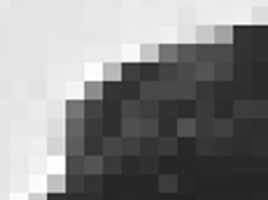
Pooling is the next thing that CNN does. The goal of pooling is to strip any not needed information from the image that we have applied the convolution operation to. Why do we need that? If you zoom in on an edge in a grayscale image, you will see that the edge itself is constructed of a bunch of different pixels – some with lighter or darker color. E.g., the edge that the network is trying to detect looks like a gradient when zoomed, so we would like to have much less of that gradient and make the edge look sharper. Here you can see that the edge consists of whiter and darker parts.

Image source

Pooling is usually performed using simple operations like Min, Max or Average, but there are more complex ones like Global Average Pooling, Fractional Pooling, Adaptive Pooling, etc.

Pooling is performed on the already generated feature map by sliding a fixed size window through the feature map and picking up the maximum values for each stride. Max pooling simply takes the highest value. Here’s a simple visual representation from Wikipedia:

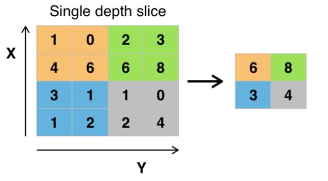
In the following example in the orange squares 6 is the largest number, so 6 is picked up. In the green squares 8 is the largest number so it is picked up and so on.

If we have done the same with the average pooling layer it would have resulted in orange: 1 + 0 + 4 + 6 = 11 and then 11 / 4 = 2.75

So Max pooling would make the features (edges, curves, etc.) stand out more, while average pooling would make the features smoother. Min pooling is used mainly when there’s a lighter background to focus on the darker pixels.

Image source

What do those neurons do?

You would probably think: How does CNN use a 1-dimensional array to make predictions? Well, applying filters is basically a way to detect specific patterns in an image. E.g. we can use a filter to detect horizontal edges, vertical edges, curves, loops and so on. This 1D array of features is the input layer which when passed to the network would cause some neurons in the first hidden layer to activate, which will activate other neurons in the next layer, and so on.  So long story short what CNN does (when it comes to image classification for example) is classify which combination of subcomponents corresponds to a specific predefined class. This might sound fuzzy now, but bear with me. Below you can see an example of a CNN with an input layer and a bunch of hidden layers (the number of hidden layers depends on the specific case, but for now let’s take as an example 2 layers) and an output layer which does the prediction.

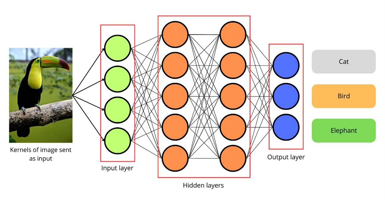
Small replica of a neural network

If we take as an example an image with 32×32 pixels (which would be of pretty low quality) it would result in 1024 individual pixels. In the case of a grayscale image each if this pixel holds a value between 0 and 255. We apply the convolution operation to the first layer (the input layer) and we get 1024 neurons which have specific activations calculated from the filter. Each neuron from the previous layer is connected to each neuron from the next layer and that connection has a specific weight. To compute the activation of a neuron in the next layer you just take the activations of all neurons from the previous layer that are connected to the specific neuron in the next layer and compute their weighted sum. The weighted sum is calculated by calculating the sum of the activation + the weight for each neuron.

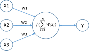
Image source

The computation of this weighted sum will result in any number, so what we would do next is use an activation function that will set a value of the neuron between 0 and 1. That way we know how “active” a neuron is (which as mentioned means how confident it is that a specific pattern presents like an edge, curve, color, etc.). We will learn more on activation functions in the next section.

For the neural network to make predictions the weights and activations in the hidden layers will need to be tweaked to help the neural network to learn, but we will learn about that in the next blogpost. As of now, if we take the current examples above, they will end up with completely random numbers.

Activation Functions

Activation functions are functions such as Sigmoid, Rectified Linear Unit (ReLU), Softmax, etc. Simply put they are used to calculate if a neuron is firing or not and how much is it firing, similarly to how biological neurons are electrically and chemically charged. What activation functions do is to squish the value of a neuron to a value between 0 or 1 (although some activation functions return values in the range of -1 to 1)

In the past Sigmoid was widely used, but now mainly ReLU and Softmax are prevailing. ReLU is usually applied inside of the hidden layer, while Softmax is used in the output layer.

Example of ReLU

The way ReLU works is it receives the weighted sum of the inputs and returns 0 if the sum is less than or equal to 0. If the input of ReLU is larger than 0 ten it just returns the input value. Here’s how ReLU looks in Python code:

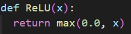
Here’s also a visual representation of how ReLU is applied in a small neural network.

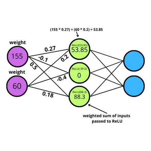
For example, the first node in the hidden layer has a value of 53.85. That is calculated as the value of the first node times the weight + the value of the second node times the weight, so that is (155*0.27) + (60*0.2) = 53.85

You can see that the second node in the hidden layer results in a value of 0 because the weighted sum of the inputs is (155 * -0.1) + (60 * -0.4) = -39.5 which ReLU will automatically set to 0 as it is a negative number.

Neurons that don’t have activation functions applied to them would output both positive and negative values. The issue here is that they would be limited to learning linear relationships, making them not that well suited for tasks that require capturing complex, non-linear features, and patterns in data.

Making predictions

In the final layer CNN main tasks is to make predictions. This is done again using an activation function, but this time the choice of activation function is different. We would use an activation function such as: Sigmoid function, Softmax, Linear/Identity and others like Gated Linear Unit (GLU) or GeLU, or others.

Softmax activation function

Softmax is usually the default choice when performing classification rather than for recognition tasks. It simply converts arbitrary values into probabilities with values between 0 and 1 (you can think of it as 0% to 100% sure to which class the image belongs to). Softmax is performed using the following steps:

1. The mathematical constant e (equal to approximately: 2.71828) is raised to the power of the sum of all probabilities. Keep in mind that currently we are talking about image classification which means that the specific neural network would try to guess which of the predefined classes the image belongs to. This first step is basically calculating the exponential raw score for a specific class.
2. Then all those exponential raw scores are summed up. This is what is called the
3. Then the exponential raw score of a specific class is divided by the denominator.

Example of Softmax

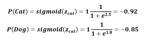
Here’s a small example: Suppose we have a CNN which should classify an image as either dog, cat, or elephant. The neural network has already run all the previous steps and has received a result of 2.5 for cat and 1.8 for dog and 0.2 for elephant. At this point we can tell that the image is a cat since cat has the largest raw score, but what Softmax gives us is probabilistic interpretation of that score, so that we know “how sure” the network is that the provided image is a specific class. This is how the formula would look like for example for cat:

So going back to the example, to get the probability score for cat we would divide(e to the power of 2.5) by (e to the power of 2.5) plus (e to the power of 1.8).

e^2.5 / e^2.5 + e^1.8 + e^0.2 = ~0.62 chance that it’s a cat.

The same is done for the raw score of the dog:

e^1.8 / e^2.5 + e^1.8 + e^0.2 = ~ 0.31 chance that it’s a dog

And for the elephant:

e^0.2 / e^2.5 + e^1.8 + e^0.2 = ~ 0.06 chance that it’s an elephant

In comparison to Softmax, Sigmoid is used mostly for binary classification, so it’s either yes or no (one or the other). Here is an example of the Sigmoid function, but this time only with cat and dog.

To sum up

In this blog post, we’ve demystified the forward propagation of Convolutional Neural Networks (CNNs), shedding light on how these neural networks power image recognition and classification. We began by simplifying the complex mechanisms behind CNNs, offering a beginner-friendly explanation. We explored the convolution operation, feature maps, pooling, and the role of neurons and activation functions in the decision-making process.

In the next chapter of our exploration, we’ll delve into the fascinating world of CNN training and optimization (a.k.a. Backpropagation), where these networks learn and refine their abilities to recognize and classify objects in images. So stay tuned for our upcoming post, as we continue our journey through the magic of image recognition with CNNs.